PINN Formulation for Grad-Shafranov

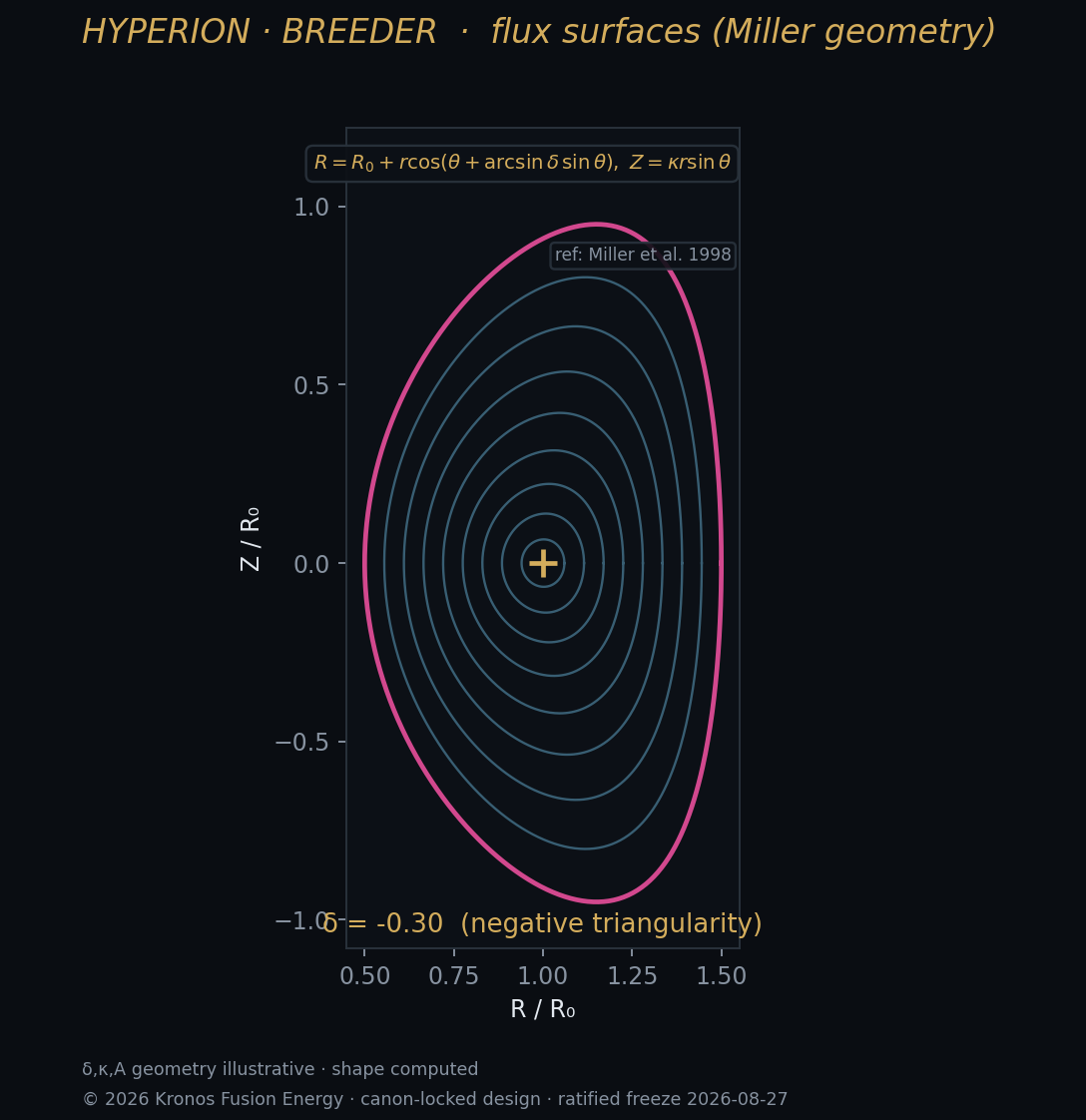
The breeder's equilibrium PINN encodes Delta* psi with the true source and negative-triangularity boundary, giving a mesh-free solver fast enough for the twin.

Setting up the equilibrium PINN

The breeder equilibrium PINN represents psi(R,Z) as a network and drives its Grad-Shafranov residual to zero over collocation points inside the plasma, while matching the negative-triangularity boundary. Because the source depends on psi through the free profiles p'(psi) and F F'(psi), the loss couples the network to those profile parameterizations.

PINN loss for Grad-Shafranov:

  L = w_pde * mean_i | Delta* psi_theta(x_i)
                       + mu0 R_i^2 p'(psi_theta)
                       + F F'(psi_theta) |^2
    + w_bc  * mean_j | psi_theta(x_j) - psi_b |^2   (LCFS, delta -0.30)
    + w_ax  * | psi_theta(x_axis) - psi_axis |^2

  Delta* from autodiff (see PINN fundamentals)

Encoding the operating point

The breeder's canonical parameters enter through normalization and the profile parameterization: 9.66 MA total current fixes the integral of J_phi, 16.84 T peak field and 8 T on-axis fix F near axis, and the boundary term carries delta -0.30. Non-dimensionalizing R, Z, and psi keeps the loss terms comparably scaled, which conditioning demands.

# equilibrium PINN training step (schematic)
def step(net, prof, coll_pts, bdy_pts):
    r_pde = gs_residual(net, coll_pts, prof.pprime, prof.ffprime)
    r_bc  = net(bdy_pts) - psi_boundary            # delta -0.30 shape
    Ip    = integrate_Jphi(net, prof) - 9.66e6     # current constraint
    L = w1*mse(r_pde) + w2*mse(r_bc) + w3*Ip**2
    return L                                       # backprop -> theta

Role in the loop

Once trained over a family of profiles and shapes, the PINN evaluates a full equilibrium in one forward pass, feeding the KRONOS-CTRL twin's MHD module inside the 1-100 ms L3 budget. It is retrained offline against the FEM solver, and its per-point residual is exposed as a confidence field so the twin can down-weight regions where the PINN is straining.

This equilibrium PINN is a design-and-simulation tool validated against FEM; it will be re-anchored to reconstructed equilibria after FOAK first tritium ~2030, but it makes no net-gain claim.

Training the profile family

The PINN is not trained on a single equilibrium but on a parameterized family: profiles p'(psi) and F F'(psi) are drawn across their admissible ranges, and boundary shape descriptors are varied around delta -0.30. The network conditions on these parameters as extra inputs, so one trained model spans the operating space rather than a single point. This is what lets the twin query equilibria for candidate scenarios without retraining.

Curriculum helps: training starts on smooth, well-behaved profiles and progressively introduces steeper edge gradients and stronger shaping, so the network builds up the hard features rather than facing them cold. The current constraint against 9.66 MA and the axis and boundary conditions are enforced throughout, keeping every intermediate model a physically admissible equilibrium.