Gyrokinetic Turbulence Simulations

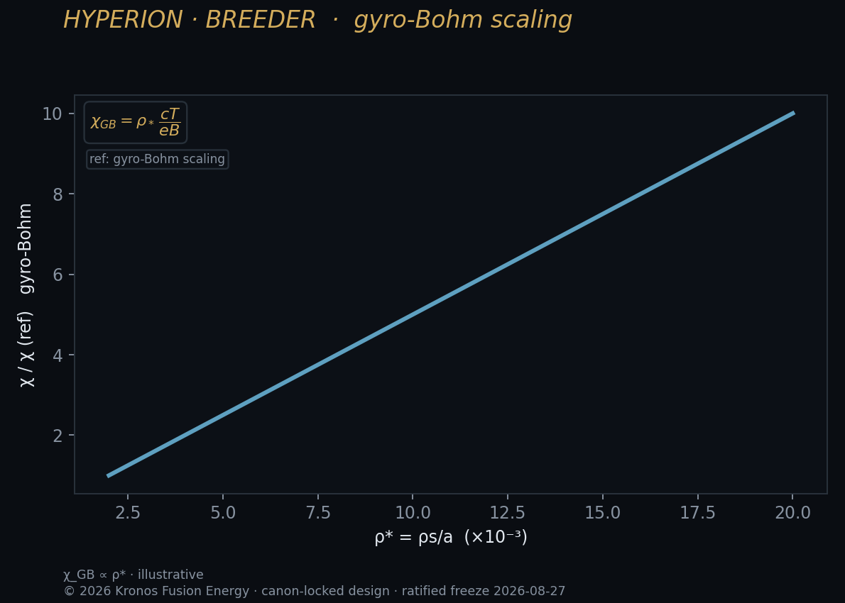
First-principles turbulence solves that supply the transport coefficients no reduced model can reliably predict for either machine.

Turbulence is the transport source

Cross-field transport in both machines is dominated by micro-turbulence driven by density and temperature gradients. Gyrokinetics is the first-principles description of that turbulence, and it is among the most compute-intensive workloads on L0. It exists to supply the diffusivities the transport solver needs but cannot invent.

Why gyrokinetic and not full kinetic

A full six-dimensional kinetic treatment of every particle orbit is intractable. Gyrokinetics averages over the fast gyration around field lines, reducing velocity space to two dimensions and removing the fastest timescale, while keeping the turbulence physics. The result is a five-dimensional distribution-function problem, still enormous but solvable on large parallel systems.

# Gyrokinetic equation (schematic, gyro-averaged f):
# df/dt + (v_par b + v_drift).grad f
#   + (q/m) E_par df/dv_par = C[f]
# 5D phase space (3 space, v_parallel, magnetic moment)
# C[f] : collision operator

How Kronos uses the output

Gyrokinetic runs produce turbulent fluxes as functions of the local gradients, from which effective diffusivities are extracted. Because the runs are costly, Kronos uses them to train and calibrate reduced models and surrogates, then uses the cheap surrogates for broad profile sweeps, reserving full gyrokinetics for anchor points and validation.

• Ion- and electron-scale turbulence drives
• Effective particle and heat diffusivities
• Calibration data for reduced transport models
• Sensitivity of confinement to gradient stiffness

For the breeder, gyrokinetics helps quantify how negative triangularity and the spherical-tokamak geometry shape turbulent transport, part of the physics case for the delta -0.30 design. For the burner, it informs central-cell transport under mirror confinement. Both machines draw on the same solver with different geometry and profiles.

These runs are strong-scaling-limited by communication, so they sit toward the coupled end of the substrate and demand low-latency interconnect. They are the clearest case where L0 pays an extreme compute cost once, offline, to buy transport knowledge that would otherwise be a guess.